Wednesday, 1 July, 2026
Spreadsheet
The IsoFind spreadsheet is an integrated calculation environment designed for isotopic data processing. It combines the functions of a standard spreadsheet with a set of native geochemical formulas and a direct connection to the project database.
Accessing the Spreadsheet
The spreadsheet is accessible from IsoFind's main side navigation bar:
Main navigation
→
Spreadsheet
On opening, an empty workbook is created automatically with a first sheet of 100 rows by 26 columns. The maximum capacity is 10,000 rows and 100 columns per sheet.
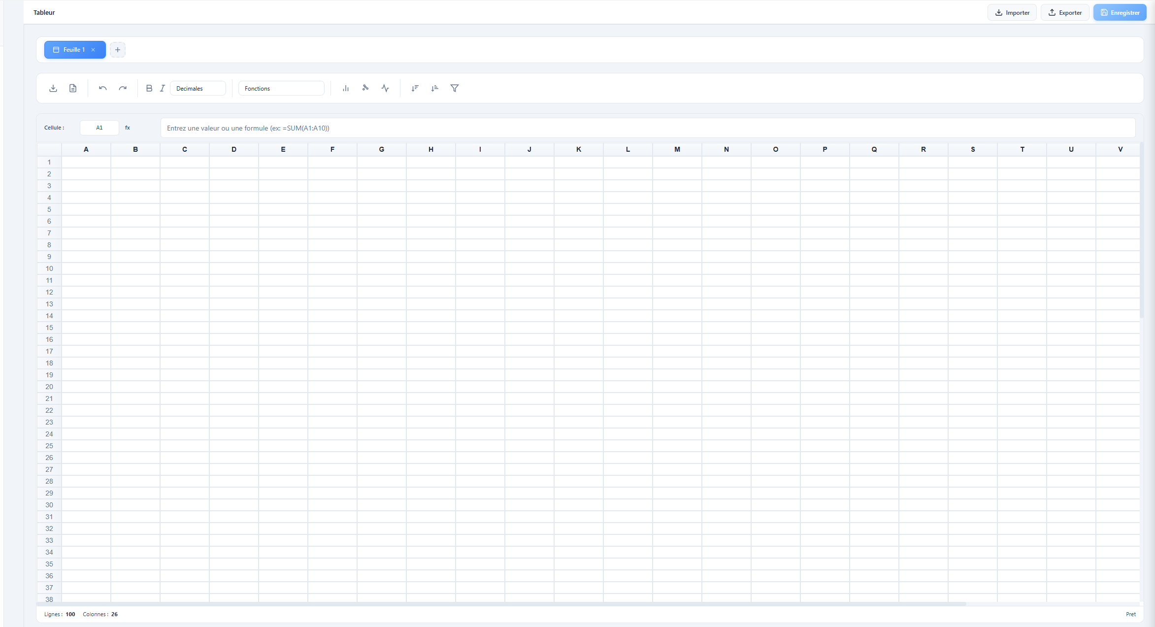 Figure 1: Spreadsheet interface with toolbar, formula bar and active sheet.
Interface Layout
The interface is divided into several distinct work areas.
Top toolbar
The toolbar groups the most frequent actions: text formatting (bold, italic), decimal rounding on the selection, ascending and descending sort, function insertion, and access to the import and chart panels.
Formula bar
The formula bar displays the reference of the active cell and its content. It allows a value or formula to be entered or modified before confirmation with the Enter key. All formulas must begin with the = sign.
Data grid
The central grid is fully editable. Columns are named with letters (A, B, C... Z, AA, AB...) and rows with integers. Rows and columns can be resized by dragging the header separators. Columns can also be reordered by drag and drop.
Sheet tabs
The tab bar at the bottom of the grid lists the workbook's sheets. Clicking the + button creates a new sheet. Double-clicking a tab name allows it to be renamed. The cross on each tab deletes the corresponding sheet (this action is irreversible; deletion of the last sheet is blocked).
Status bar
The bottom bar permanently displays the number of rows and columns in the active sheet. When a range of numeric cells is selected, it automatically displays the sum, average, minimum, maximum and count of values in the selection.
Importing Data
The spreadsheet offers two distinct import sources, accessible via the Import button in the toolbar.
Toolbar
→
Import
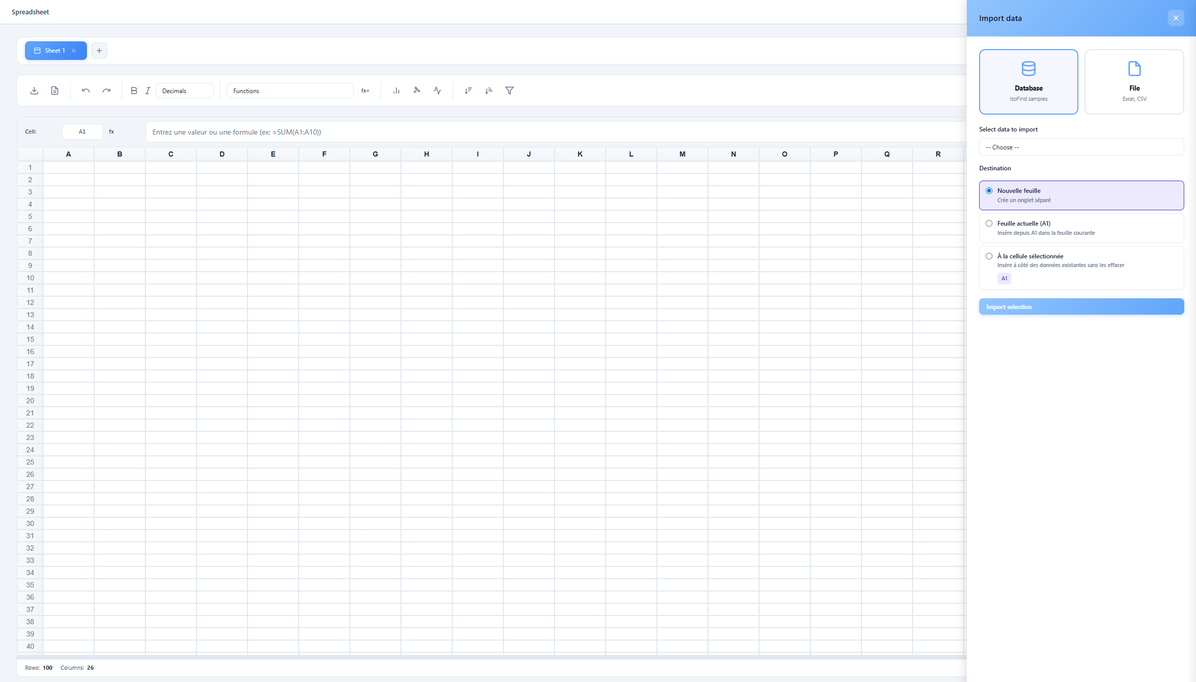 Figure 2: Import panel with the two available sources.
Import from the database
This source queries the IsoFind database of the current project directly. Four types of data can be extracted:
| Type | Imported content |
|---|---|
| Samples | Metadata only (name, material type, GPS coordinates, collection date, project, sector, classification, description). |
| Isotopic data | Measured isotopic ratios with their uncertainties (2σ), filtered by element or material type. |
| Complete data | Merge of metadata and isotopic measurements into a single structured table. |
| Applied methods | Analytical pipelines associated with samples (feature currently under development). |
The list of available samples is displayed with a name search field and filters by material type and isotopic element. A checkbox allows the entire result set to be selected in a single action.
Import format for isotopic data
For imports of type Isotopic data or Complete data, IsoFind offers three layout modes:
| Mode | Structure of the resulting table |
|---|---|
| Automatic | IsoFind analyses the data and chooses the extended format if the same sample has multiple measurements of the same ratio, otherwise the compact format. |
| Compact | One row per sample. Each ratio occupies a column, and the associated uncertainty occupies the next column. |
| Extended | One row per individual measurement. Discriminating columns (date, matrix type, standard used...) are added automatically to differentiate multiple measurements of the same sample. The value column is named after the isotopic ratio (e.g. 206Pb/204Pb) rather than the generic "Value". |
In automatic mode, IsoFind detects fields that vary between multiple measurements of the same sample (collection date, matrix type, element, ratio, standard) and only includes the columns that are effectively discriminating. This guarantees a minimal but complete table.
Import destination
Each import offers three destination options, accessible at the bottom of the panel:
| Destination | Behaviour |
|---|---|
| New sheet | Creates a new tab in the workbook and inserts the data there. Default behaviour. |
| Current sheet (A1) | Inserts the data from cell A1 of the active sheet, without creating a new tab. |
| At selected cell | Inserts the data from the active cell at the time the panel was opened, without erasing existing data. Allows multiple tables to be placed side by side on the same sheet. |
To import two tables side by side (e.g. two different isotopic ratios), select the starting cell of the second table in the grid, open the import panel, then choose At selected cell. The target cell is displayed in a real-time badge in the panel.
Import from a file
The second source allows an external file to be loaded by click or drag and drop. Accepted formats are:
| Format | Behaviour |
|---|---|
| .xlsx / .xls | Each sheet of the Excel file is imported into a separate sheet in the IsoFind workbook. The first sheet can be inserted into the active sheet. |
| .csv | The file is parsed with automatic detection of comma and semicolon separators. An option allows the first row to be treated as a header. Double quotes are handled correctly. |
| .isosheet | Native IsoFind format. Reloads the entire workbook (all sheets, formulas and metadata) in the exact state in which it was saved. |
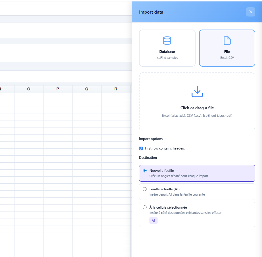 Figure 3: Drop zone for importing external files.
Auto-Save and Session Restoration
The spreadsheet automatically saves the workbook state to the browser's local storage. This save is transparent and requires no user action.
How it works
A save is triggered automatically three seconds after each modification (keystroke, import, formula). A second pass every thirty seconds catches any modifications not yet saved. The time of the last auto-save is displayed in the status bar.
Restoration on return
Each time the spreadsheet is opened, if a previous session exists, a restoration banner appears at the bottom of the screen. It shows the workbook name, the date and time of the last save, and the number of sheets.
| Action | Result |
|---|---|
| Restore | Loads the workbook in the exact state of the last auto-save. |
| Dismiss | Deletes the save and starts with an empty workbook. |
Auto-save uses the browser's local storage. It is independent of manual saving in .isosheet format, which remains the only way to transfer a workbook between machines or to preserve it permanently.
Formulas and Calculations
The spreadsheet supports standard formulas (SUM, AVERAGE, MIN, MAX, IF, etc.) as well as a set of geochemical and statistical formulas developed specifically for IsoFind.
Entering a formula
Any formula is entered in a cell or in the formula bar by starting with =. Selecting a range before using the function insertion button automatically fills the range as the argument.
Isotopic statistical formulas
| Formula | Syntax | Description |
|---|---|---|
| WMEAN | WMEAN(values, uncertainties) | Weighted mean by analytical uncertainties. Formula: Σ(xᵢ/σᵢ²) / Σ(1/σᵢ²). |
| WMEAN_ERROR | WMEAN_ERROR(uncertainties) | Standard error of the weighted mean: 1 / √Σ(1/σᵢ²). |
| MSWD | MSWD(values, uncertainties) | Mean Square Weighted Deviation. Measures the scatter of data relative to analytical uncertainties. An MSWD close to 1 indicates scatter compatible with the uncertainties. |
| STDERR | STDERR(values) | Standard error of the mean (standard deviation / √n). |
| MEDIAN | MEDIAN(values) | Median of the distribution, robust to outliers. |
| MAD | MAD(values) | Median Absolute Deviation, a robust dispersion indicator. |
Geochemical formulas
| Formula | Syntax | Description |
|---|---|---|
| DELTA | DELTA(ratio, standard) | Delta (δ) notation in per mille: ((ratio/standard) - 1) × 1000. |
| DELTA_TO_RATIO | DELTA_TO_RATIO(delta, standard) | Inverse conversion from delta notation back to the absolute ratio. |
| EPSILON_ND | EPSILON_ND(¹⁴³Nd/¹⁴⁴Nd, [CHUR]) | Calculation of εNd relative to CHUR (default value: 0.512638). Formula: ((sample/CHUR) - 1) × 10000. |
| MASS_BIAS_EXP | MASS_BIAS_EXP(measured, reference, mass_ratio) | Mass bias coefficient using the exponential law. |
| INITIAL_SR | INITIAL_SR(⁸⁷Sr/⁸⁶Sr, ⁸⁷Rb/⁸⁶Sr, age_Ma) | Initial ⁸⁷Sr/⁸⁶Sr ratio at a given age. Uses λRb = 1.42 × 10⁻¹¹ /yr. |
Geochronological formulas
| Formula | Syntax | Description |
|---|---|---|
| ISOCHRON_AGE_RB_SR | ISOCHRON_AGE_RB_SR(slope) | Rb-Sr isochron age in millions of years. λRb-87 = 1.42 × 10⁻¹¹ /yr. |
| ISOCHRON_AGE_SM_ND | ISOCHRON_AGE_SM_ND(slope) | Sm-Nd isochron age in millions of years. λSm-147 = 6.54 × 10⁻¹² /yr. |
| AGE_U_PB | AGE_U_PB(²⁰⁶Pb/²³⁸U) | U-Pb age in millions of years. λU-238 = 1.55125 × 10⁻¹⁰ /yr. |
Regression formulas
| Formula | Syntax | Description |
|---|---|---|
| SLOPE | SLOPE(x, y) | Slope of the least-squares linear regression. |
| INTERCEPT | INTERCEPT(x, y) | Y-intercept of the linear regression. |
| R_SQUARED | R_SQUARED(x, y) | Coefficient of determination R² of the regression. |
| SLOPE_ERROR | SLOPE_ERROR(x, y) | Standard error on the regression slope (requires at least 3 points). |
Error propagation formulas
| Formula | Syntax | Description |
|---|---|---|
| ERROR_ADD | ERROR_ADD(err1, err2, ...) | Error propagation for a sum or difference: √(σ₁² + σ₂² + ...). |
| ERROR_MUL | ERROR_MUL(value, rel_err1, rel_err2, ...) | Error propagation for a product or quotient in terms of relative errors. |
| TO_2SIGMA | TO_2SIGMA(uncertainty_1sigma) | Conversion of a 1σ uncertainty to 2σ. |
| TO_1SIGMA | TO_1SIGMA(uncertainty_2sigma) | Conversion of a 2σ uncertainty to 1σ. |
| TO_RELATIVE | TO_RELATIVE(value, absolute_error) | Conversion of an absolute error to a relative error (in percent). |
| TO_ABSOLUTE | TO_ABSOLUTE(value, relative_error) | Conversion of a relative error to an absolute error. |
Isotopic reference standard
The GET_STANDARD formula retrieves the reference ratio value of an international isotopic standard directly into a cell:
GET_STANDARD("NIST614", "206Pb/204Pb") returns the certified reference value for this ratio in this material. The list of available standards can be consulted via the ISOTOPE_STANDARDS constant.
Custom formulas
It is possible to define your own calculation formulas and reuse them in any cell of the workbook. The custom formula manager is accessible from the toolbar:
Toolbar
→
My formulas...
 Figure 4: Interface for creating and testing a custom formula.
Each custom formula is defined by a name, a mathematical expression using the variables x, y and z, and an optional description. Standard mathematical functions are available in expressions: Math.sqrt, Math.pow, Math.log, Math.exp, Math.abs, etc.
An integrated test tool allows the result of the expression to be verified with arbitrary values of x, y and z before saving the formula. Custom formulas are stored locally and persist between sessions.
Creating Charts
The chart panel is accessible from the toolbar or from the context menu of a selection. Nine chart types are available, covering common needs in isotopic geochemistry.
Toolbar
→
Chart
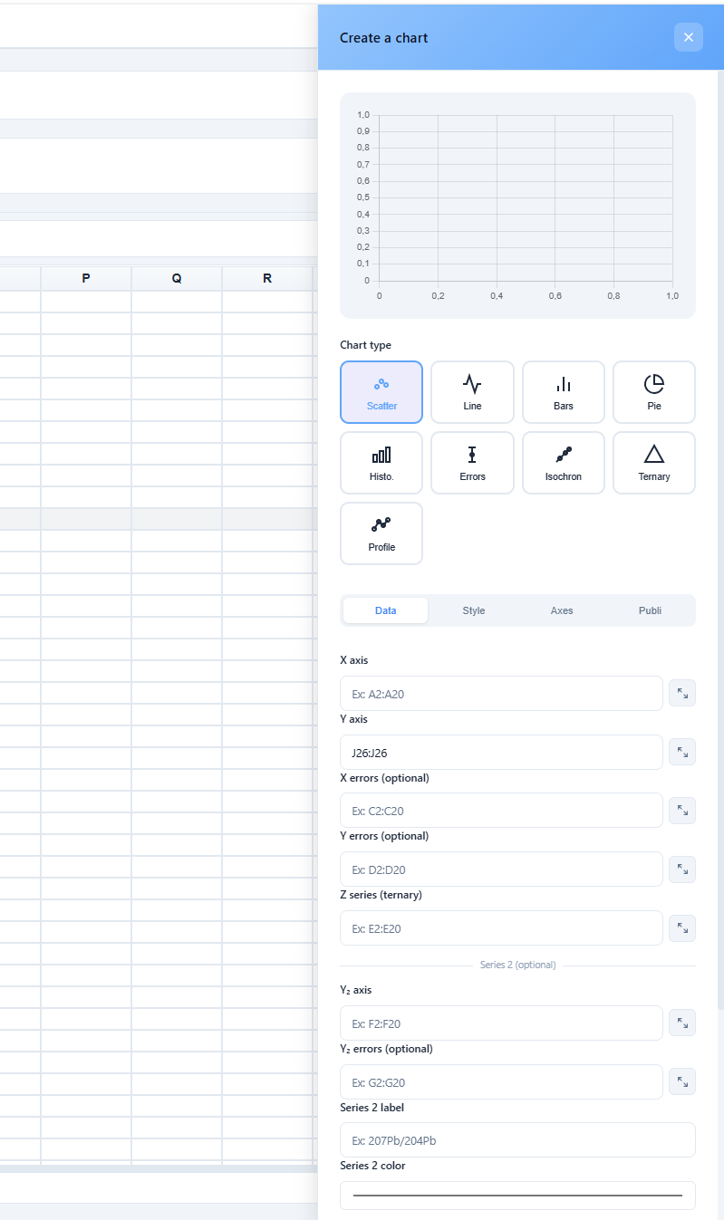 Figure 5: Chart configuration panel with real-time preview.
Available chart types
| Type | Typical use |
|---|---|
| Scatter plot | Binary isotopic diagrams, correlations between ratios. |
| Line chart | Time series, fractionation profiles. |
| Bar chart | Value comparison between samples or groups. |
| Pie chart | Proportional breakdown. |
| Histogram | Frequency distribution of a ratio or value. |
| Error bars | Representation of values with their analytical uncertainties. |
| Isochron | Isochron diagram with automatic linear regression. Axes are pre-labelled for Rb-Sr and Sm-Nd systems. |
| Ternary | Three-component diagram. Requires definition of an X, Y and Z range. |
| Categories | Visualisation of values grouped by sample categories. |
Selecting data ranges by drag
Each data field in the chart panel (X axis, Y axis, X errors, Y errors, Z series, Series 2, Labels) has a targeting button represented by a cursor icon. This button allows the corresponding range to be defined directly by selection in the grid, without manually entering the reference.
The procedure is as follows: click the targeting button for the desired field, drag over the cells to use, then release. The range reference is automatically injected into the field, and the chart preview updates immediately. An indigo banner at the top of the Data tab signals the active capture mode; it can be cancelled by clicking the cross or clicking the button again.
Data fields can mix manual entry and drag selection. For example, the X range can be entered manually while the Y errors range is defined by drag.
Multiple series and sample names
The Data tab includes a Series 2 section allowing a second Y dataset to be overlaid on the same chart, with its own colour, uncertainties and legend label. Both series share the same X axis.
A Labels (tooltip) section allows a column of sample names to be associated with the chart's data points. When a range is defined in this field, hovering over a point displays the corresponding sample name in the tooltip, in addition to the coordinates and uncertainty. If the field is left empty, IsoFind attempts to automatically detect a column whose header matches Sample, Nom, ID, Label or Site.
Chart configuration
If a range is selected when the panel is opened, the X and Y data ranges are pre-filled automatically. The panel provides a real-time preview updated on every modification. When creating an error bars chart, IsoFind automatically detects uncertainty columns if they are named with the suffix (2σ).
Managing created charts
Created charts are listed in the My charts tab of the panel. Each chart can be downloaded as a PNG file. The Preview tab allows the preview of the chart currently being configured to be consulted before confirming.
Publication-Ready Charts (Publi Tab)
The Publi tab of the chart panel groups the advanced formatting options designed to produce figures directly usable in a scientific article.
Chart panel
→
Publi tab
Figure format
Six dimension presets corresponding to the templates of the main journals are available. Selecting a preset automatically fills the width and height fields; the values remain manually editable.
| Preset | Dimensions | Use |
|---|---|---|
| Nature — 1 column | 86 mm | Single-column figure for Nature, Science, Cell. |
| Nature — 2 columns | 180 mm | Full-width double-column figure. |
| Science — 1 column | 90 mm | Science single-column template. |
| EPSL / GCA | 190 mm | Elsevier geochemistry journals (EPSL, GCA, Chemical Geology...). |
| Square | 150 × 150 mm | Generic square format. |
| Custom | Free | Manual entry of width and height in pixels. |
Typography
Four font families are available, covering the main scientific editorial conventions. Sizes are independently adjustable for the title, axis labels and tick marks.
| Font | Typical use |
|---|---|
| Helvetica / Arial | Default. Suitable for most sans-serif journals. |
| Times New Roman | Nature, Science and journals requiring a serif font. |
| Georgia | Readable serif alternative at small sizes. |
| Arial Narrow | Space-saving for dense legends. |
Colour palettes
Five predefined palettes are available. Selecting a palette automatically applies the colours to the chart series and updates the colour pickers in the Style tab.
| Palette | Description |
|---|---|
| Custom colours | Uses the colours defined in the Style tab. |
| Colour-blind safe (Wong 2011) | 8 colours distinguishable by all forms of colour blindness. Recommended for any publication. |
| Greyscale | For journals or supplements in black and white. |
| Viridis | Perceptually uniform, colour-blind compatible palette. |
| Geochemistry tones | Ochre, rust and blue palette, suited to conventional isotopic representations. |
Advanced axes
Additional options allow fine control of axis rendering: forced number of tick marks on X and Y, display of a zero line, full frame (top and right borders, publication style), and secondary grid.
Annotations
The Publi tab provides an annotation system for adding graphical elements directly on the chart. Five types are available:
| Type | Description |
|---|---|
| Text | Label positioned at given coordinates (axis units, not pixels). |
| Arrow + text | Arrow connecting an origin point to a target point, with optional label. |
| Ellipse | Ellipse centred on a point, useful for delimiting a group of samples. |
| Horizontal line | Dashed line spanning the full width of the chart at a given Y value. |
| Vertical line | Dashed line spanning the full height of the chart at a given X value. |
Each annotation is defined by its coordinates in axis units (not pixels), a colour and a font size. Annotations are listed with an individual delete button and rendered in real time in the preview.
Coordinates can be entered manually or placed by clicking directly on the chart: activate the Click button, then click on the chart to pre-fill the X and Y fields. If text is already entered, the annotation is added immediately; otherwise, the coordinates are pre-filled for manual confirmation.
Annotations use axis coordinates (real isotopic values). They therefore remain correctly positioned if the axis scale or limits are modified afterwards.
Publication export
| Format | Description |
|---|---|
| Vector SVG | SVG export, infinitely scalable without loss. Usable in Inkscape, Illustrator or directly in LaTeX. |
| PNG 300 dpi | The chart is natively reconstructed in a high-resolution canvas (×3.125 relative to screen display). All elements — text, lines, points, annotations — are rendered vectorially, without bitmap upscaling. |
Saving and Exporting
Saving the workbook
Workbook saving is accessible via the Save button in the toolbar or with the keyboard shortcut Ctrl + S.
Toolbar
→
Save
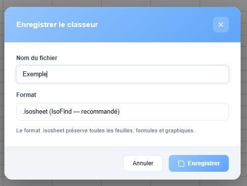 Figure 6: Name and format selection window for saving.
Three formats are available for saving:
| Format | Description |
|---|---|
| .isosheet (recommended) | Native IsoFind format. Preserves all sheets, formulas, charts and workbook metadata. Structured JSON file fully reloadable. |
| .xlsx | All sheets are exported to a compatible Excel file. IsoFind-specific formulas are not interpretable outside the spreadsheet. |
| .csv | The active sheet only is exported as comma-delimited text. |
Data export
The export function provides finer control over the content to extract:
Toolbar
→
Export
Four export formats are available: Excel (.xlsx), CSV (.csv), JSON (.json) and PDF (.pdf, currently under development). For each, it is possible to choose between exporting all sheets, the active sheet only, or the current selection.
JSON export produces the complete workbook representation (data, columns, styles, metadata), which can serve as an interface with Python scripts or external pipelines.
Keyboard Shortcuts
| Shortcut | Action |
|---|---|
| Ctrl + S | Opens the workbook save window. |
| Ctrl + Z | Undoes the last action. |
| Ctrl + Y | Redoes the last undone action. |
| Ctrl + B | Applies or removes bold formatting on the selection. |
| Ctrl + I | Applies or removes italic formatting on the selection. |
| Enter in the formula bar | Confirms the formula or value entered in the active cell. |
Limitations and Technical Considerations
The IsoFind spreadsheet runs entirely client-side, with no automatic synchronisation with the database. Modifications made in the spreadsheet do not alter data saved in IsoFind: the spreadsheet is an independent analytical workspace.
The maximum capacity per sheet is 10,000 rows and 100 columns. For larger volumes, it is advisable to distribute data across multiple sheets or to use the IsoFind API for programmatic processing.
The .isosheet format is the only save format that guarantees complete workbook restoration, including custom formulas active at the time of saving. The .xlsx and .csv formats only retain calculated values.